|
ABF305 Investment Management
Lecture 13
In this lecture, we will:
在本次讲座中,我们将:
Cover risk aversion and capital allocation to risky assets:
包括风险规避风险资产和资本分配:
Read Chapter 6 in the textbook.
阅读教科书中的第6章
You do not have to read, however, pages 161-165, namely the section on estimating risk aversion.
你不必阅读,然而,第161-165页,即估计风险厌恶情绪的部分。
Just to completely confuse you, do read, however, the section Words from the street’ part on page 162-163. It is titled ‘Time for Investing’s four-letter word’.
只是完全迷惑你,不要读,但是,节词从街道'部分第162-163页。它的标题是“时间投资的四个字母的单词”。
‘Modern Portfolio Theory’ addressed by academics (e.g.Markowitz and Sharpe).
现代投资组合理论解决的学者(如Markowitz和夏普)。
Assumptions:
假设:
Investors will avoid risk unless they can anticipate a reward for engaging in risky investments.
投资者将规避风险,除非他们能预见从事风险投资的奖励。
Investor’s have a ‘utility function’.
投资者的“效用函数”。
What do we mean by risk aversion?
规避风险是什么意思?
Quantifying risk tolerance arises from quantifying the psychological behaviour of people and their money habits through a series of questions. This is achieved through such questionnaires as those on page 162 in your textbook.*
来自量化的风险承受能力的一系列问题,通过量化的心理行为的人,他们的用钱习惯。这是通过问卷那些在你的教科书第162页上。
Utility Function:
应用函数
Utility is the measure of the welfare or satisfaction of an investor, (Bodie, Kane and Marcus, ‘ Investments’ 8th Edition).Welfare means benefit
Utility value is the welfare a given investor assigns to an investment with a particular return and risk, (Bodie, Kane and Marcus, ‘ Investments’ 8th Edition).
The personal utility function is the quantification between an investor’s personal trade-off between portfolio risk and expected return (Bodie, Kane and Marcus, ‘ Investments’ 8th Edition). *
Where E(r) is the expected rate of return, σ² represents the variance or stock volatility, ‘A’ denotes the risk aversion of an investor where a higher aversion is a higher value of A;
The value of a half is employed purely for scaling convention.*
We can see that the utility value is a function of the risk aversion of an investor and the stock risk.
What is the whole point of this?
The ‘utility’ score is employed to evaluate alternative portfolio choices.
Example:

We are provided with the following information:
If we have three investors with a risk aversion (A) of respectively 2.0, 3.5, and 5.0, then the utility value for each investor for each portfolio is:
For the first investor with aversion 2.0:
U= 0.07 – (1/2 x 2.0 x (.05²)) =0.0675
U= 0.09 – (1/2 x 2.0 x (0.10²)) = 0.08
U= 0.13 – (1/2 x 2.0 x (0.20²)) = 0.09
For the second investor with aversion 3.5:
U= 0.07 – (1/2 x 3.5 x (.05²)) =0.0656
U= 0.09 – (1/2 x 3.5 x (0.10²)) = 0.0725
U= 0.13 – (1/2 x 3.5 x (0.20²)) = 0.06
For the third investor with aversion 5.0:
0.07 – (1/2 x 5.0 x (.05²)) =0.0638
0.09 – (1/2 x 5.0 x (0.10²)) = 0.065
0.10 0.13 – (1/2 x 5.0 x (0.20²)) = 0.03
What are we trying to achieve ultimately?
The utility function will help us to choose a portfolio, but there are still quite a few decisions which we still need to make.
One such decision is how much capital to allocate across a risky portfolio and a risk-free asset.
What do we want.
Optimal risky portfolio is an investor’s best combination of risky assets to be mixed with safe assets to form the complete portfolio.
Optimal return relative to risk. *
Where:
the proportion of capital allocation in the risky portfolio is denoted by the letter y;
the proportion of capital in the risk free asset is denoted by (1-y);
the rate of return of the portfolio is rp;
the return on the risk free asset is rf.*
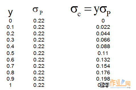
If the standard deviation for the complete portfolio (σc) is equal to the standard deviation for the risky asset portfolio (σp) multiplied by the proportion of capital allocation in that portfolio (y), namely,
With the information provided, it is possible to construct a capital allocation line (CAL).*

Example:
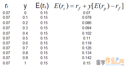
If E(rp) = 15%,
σp =22%
risk-free rate rf =7%
We change the capital allocation from 100% in the risk free asset to 100% in the risky portfolio with a 10% incremental change.
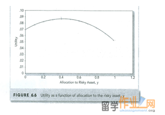
Then the capital allocation line may be denoted by the next graph.
Where ‘Y’ is the allocation in the risky portfolio.

It is also possible to use a formulae to find the optimal proportion (y*):
where y* is the proportion invested in the risky portfolio and (1-y) is the proportion invested in the risk free asset. E(rp) is the expected return on the risky portfolio, rf is risk free return, A is the investors risk aversion, and is the risky portfolio variance.

Summary of what we know:
We can quantify utility value.
We can use the utility value to arrive at an optimal capital asset allocation.
We don’t as yet know, within an asset class, the ‘optimal’ specific security choices. We will cover that in the lectures to come.
|


